

In this article, we're diving deep into a captivating lane detection algorithm I've been experimenting with. 🚗 We'll analyze a basic video, pinpoint the lane, and craft a red overlay for both left and right lanes. 🎨
Get ready for a tech journey as we explore Python's computer vision tools, led by OpenCV, alongside the dynamic duo, numpy, and matplotlib. 💻
Computer vision? It's the art of finding order in image chaos. 🧙♂️ We'll conjure magic with OpenCV, and you can run this code in any Python-friendly environment. 📦
By the end, you'll wield the power to create your own lane detection masterpiece! 🛣️

📕Solving one step at a time
First things first, let's keep it simple! 😊
One easy way to tackle this is by starting with just one image. 📷 After all, a video is just a bunch of images stitched together, right? So, let's first figure out our solution for this single image.
For instance, consider this snapshot: 📸

In the picture above, the lane markers are super clear to anyone, right? 🛣️ We humans do this without even thinking, and once we've learned to drive, spotting the lane becomes second nature. Plus, we effortlessly spot all sorts of other stuff in the scene: cars, the road's edge, signs, and even those mountains way out there. 🚗🌄 But guess what? Among all these things, the lane markers are some of the simplest to spot!
Knowing how to drive gives us a bunch of clues about lanes, making it even simpler. For example, we can guess that lanes usually run parallel to our direction, so their lines kind of slope inwards. Also, those lines never quite reach the horizon, either fading away into the distance or getting hidden by something else in the picture.
Now, let's get practical! To start our project, we'll begin by doing something straightforward: cutting out the parts of the image that we know won't have any lane info. 📷✂️
📕Cropping our Region of interest
📗Loading an Image into Memory
The very first thing we must do before we can process an image is… read an image! The following snippet can be used to load an image from a file into an array of image data which can be manipulated in Python:
import matplotlib.pyplot as plt
import matplotlib.image as mpimg
# reading in an image
image = mpimg.imread('sample.jpg')
# printing out some stats and plotting the image
print('This image is:', type(image), 'with dimensions:', image.shape)
plt.imshow(image)
plt.show()
In this code, we import the necessary library modules, load an image into memory, print some stats about the image, and display it in a plot, as below:

Awesome! 🙌 We've got an image loaded up in our Python script now. 🐍 It's like digital clay in our hands! 🖼️ This picture is sized at 1080 pixels tall, 1920 pixels wide, and has 3 colour channels for all those pretty colours. 🌈 This image is gonna be our guinea pig for testing our cool algorithm in this post. 🐹
📗Defining the Region of Interest
So, first things first, we need to pick out the part of the picture we care about. 🖼️
Now, you know how math usually starts with the origin (that's the point (0,0)) in the bottom left corner? Well, computer graphics decided to be a bit different and put the origin in the upper left corner! 🤨 But don't worry, it won't mess things up too much. Just remember, when we talk about y-coordinates, we're measuring from the top of the image, not the bottom.
Our goal is to frame the lane lines perfectly. So, to do that, we'll make a simple triangle. It starts at the bottom left corner, then goes to the middle where the horizon is, and finally, it wraps up at the bottom right corner. 🚗🔼
Here's where those points are: 👇
Bottom left: (0, 540)
Horizon: (910, 540)
Bottom right: (1920, 1080)
Easy, right? 😄
region_of_interest_vertices = [
(0, height),
(width / 2, height / 2),
(width, height),
]
📗Cropping the Region of Interest
To do the cropping of the image, we’ll define a utility function region_of_interest():
import numpy as np
import cv2
def region_of_interest(img, vertices):
    # Define a blank matrix that matches the image height/width.
    mask = np.zeros_like(img)
    # Retrieve the number of color channels of the image.
    channel_count = img.shape[2]
    # Create a match color with the same color channel counts.
    match_mask_color = (255,) * channel_count

    # Fill inside the polygon
    cv2.fillPoly(mask, vertices, match_mask_color)

    # Returning the image only where mask pixels match
    masked_image = cv2.bitwise_and(img, mask)
    return masked_image
Then we’ll run the cropping function on our image before showing it again (output below):
import matplotlib.pyplot as plt
import matplotlib.image as mpimg
region_of_interest_vertices = [
    (0, height),
    (width / 2, height / 2),
    (width, height),
]
image = mpimg.imread('sample.jpg')
cropped_image = region_of_interest(
    image,
    np.array([region_of_interest_vertices], np.int32),
)
plt.figure()
plt.imshow(cropped_image)
plt.show()

📕Detecting Edges in the Cropped Image
Now, we've got ourselves a neatly cropped image in less than 20 lines of code! 🎉 What's even cooler is that we've done it using a basic shape, and guess what? We've pretty much zapped away everything that's not related to the lane or those lane lines. 🧙♂️✨
Next up, we're diving into the exciting world of edge detection in our cropped image. 🚀 Now, there's a bit of math in this part, but don't worry, I won't get all super-technical on you. If you're curious, though, you can click the links I've added to learn more. 🤓🔍
📗Mathematics of Edge Detection
Let's make this easy-peasy! 🤓
So, here's a question to wrap our heads around edge detection: 🤔
When we look at the numbers in an image (it's like a big grid of numbers, you know), what really tells us, "Hey, there's an edge here!"?
Now, check out this lane marking 👇. See how it's got this highlighted part showing the edge's "steepness"?
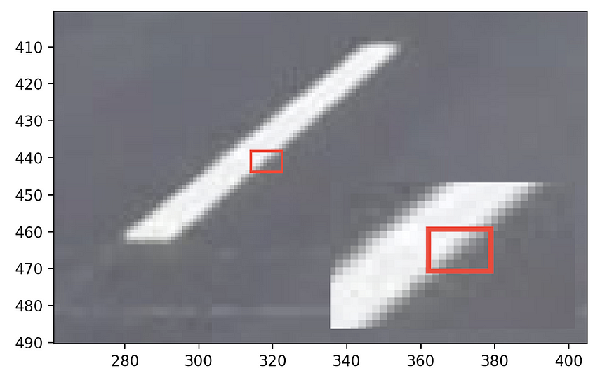
Well, if we peek at the numbers around this edge, it's pretty clear that edges are just spots where the colours change super fast. 🌈 So, when a pixel doesn't quite match the colours of its buddies, that's our cue that there's an edge.
Good news! We can totally solve this math problem. 🧮 A smarty named John F. Canny came up with an algorithm for it. He used some fancy math called "calculus of variations." 📚✍️ For those of you who've dabbled in calculus, it's basically about finding spots in the image where the colours change a lot. Canny also threw in a couple of "how strong should an edge be?" rules, but we won't dive into those here. 🤷♂️
📗Grayscale Conversion and Canny Edge Detection
Guess what? We don't really care about all those fancy colours in the picture 🌈, just how bright or dark stuff is. To keep things simple, we're going to turn the image grayscale. That's like taking out the colours and replacing them with shades of grey. 🎨➡️🖤
Now, our plan is to let Canny Edge Detection do the heavy lifting. It'll spot places where the brightness changes a lot, making them pop as edges. 🧐
And here's the best part - we don't even have to write this algorithm ourselves! 🤓 OpenCV has it ready to roll with just one command. So, let's fire up Canny Edge Detection on our cropped image with some sensible starting settings and see what it finds! 🔍
# Convert to grayscale here.
gray_image = cv2.cvtColor(cropped_image, cv2.COLOR_RGB2GRAY)
# Call Canny Edge Detection here.
cannyed_image = cv2.Canny(gray_image, 100, 200)
plt.figure()
plt.imshow(cannyed_image)
plt.show()
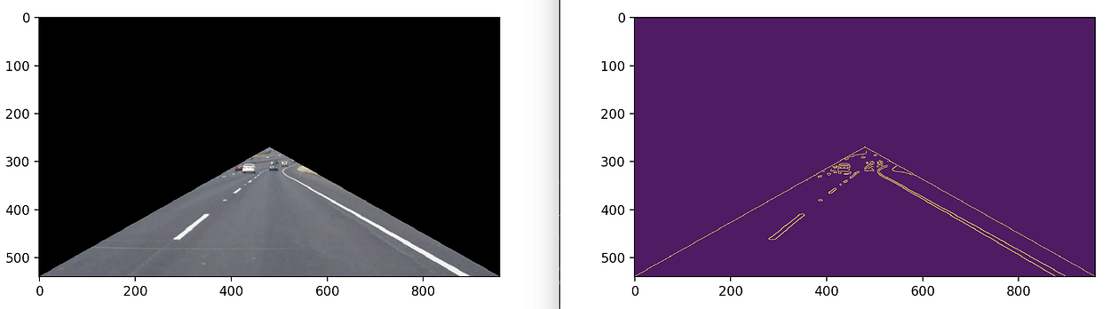
We did it! The image now contains only the single pixels which are indicative of an edge. But there’s a problem… We accidentally detected the edges of our cropped region of interest! Not to worry, we can fix this problem by simply placing the region of interest cropping after the Canny process in our pipeline. We also need to adjust the region of interest utility function to account for the fact that our image is now grayscale:
def region_of_interest(img, vertices):
    mask = np.zeros_like(img)
    match_mask_color = 255 # <-- This line altered for grayscale.

    cv2.fillPoly(mask, vertices, match_mask_color)
    masked_image = cv2.bitwise_and(img, mask)
    return masked_image
region_of_interest_vertices = [
    (0, height),
    (width / 2, height / 2),
    (width, height),
]
image = mpimg.imread('sample.jpg')
plt.figure()
plt.imshow(image)
plt.show()
gray_image = cv2.cvtColor(image, cv2.COLOR_RGB2GRAY)
cannyed_image = cv2.Canny(gray_image, 100, 200)
# Moved the cropping operation to the end of the pipeline.
cropped_image = region_of_interest(
    cannyed_image,
    np.array([region_of_interest_vertices], np.int32)
)
plt.figure()
plt.imshow(cropped_image)
plt.show()
📕Generating Lines from Edge Pixels
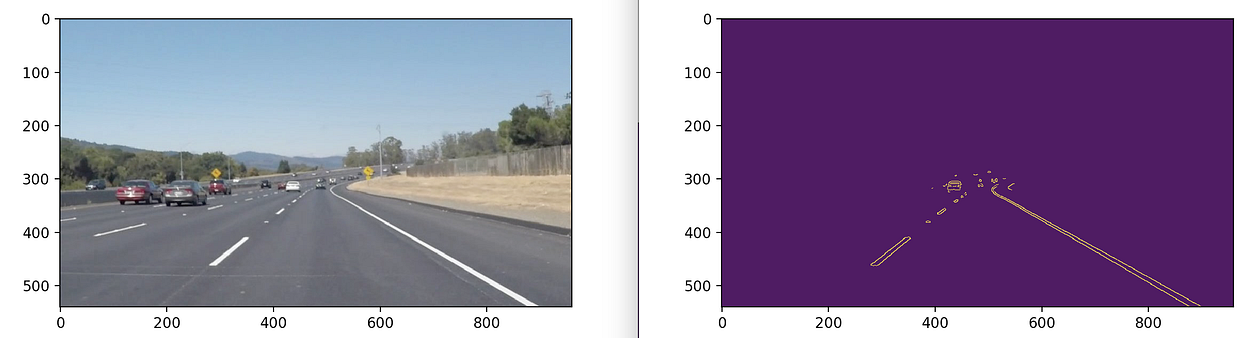
Nailed it! 👏 This seems like a solid beginning to spot those lane lines. If you check out our output pic, you'll notice that the standout stuff is definitely the lane markings. 🛣️
Now, here's the fun part. We've got these pixels that show us where the edges are, but we need to connect them to make actual lines. Sounds fancy, right? Well, the good news is, we've got some math magic to solve this. ✨ But don't sweat it; I'll keep it simple unless you want to dive deep into the details!😅🔍
📗Mathematics of Line Detection
Let's make this math thing super simple! 🤓
So, remember when we asked what defines an edge? Well, now we're wondering what makes a line. 🤔
Imagine this: We've got a picture with lots of empty spots and a bunch of 'edge pixels' that don't seem to have any pattern. But guess what? To us humans, they look like lines! 📏
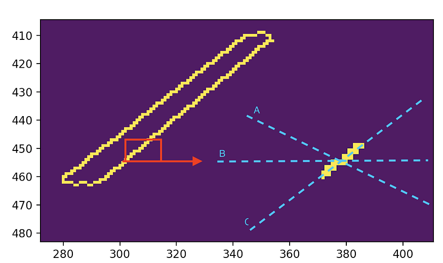
Now, if we look closely at what's going on in that liney part, those edge pixels share something cool. It's like they all agree on a few lines they could belong to. These lines are like candidates for the real line (if there is one) that passes through those edge pixels.
But here's the thing, there are so many lines we could pick! 🤯 So, we need some math tricks to narrow it down to just one line for each set of edge pixels.
Here's the hero of our story: the Hough Transform. It's like magic! 🎩✨ With this trick, we change our edge pixels into a different kind of math thing. Each edge pixel becomes a line or curve in a special space called "Hough Space." 🪄 In this space, each line represents a point in our picture, and each point represents a line in our picture. Crazy, right? 🤪
Don't worry about the math nitty-gritty; just know that this makes our problem super easy. Now, we don't have to find a line that goes through all the nearby edge pixels. Nope, we just look for where lines in Hough Space intersect. That tells us where we've got a line with enough edge pixels in our picture. 🚀🔍
We can tweak some settings to decide which lines are real and which are just noise, but let's not get bogged down in the details. 😅🔧
📕Using Hough Transforms to Detect Lines
Good news! OpenCV makes detecting lines a piece of cake! 🍰 It comes with this cool function that uses the Hough Transform to find lines in an image with edge pixels. 🪄
So, we'll give it a go on our image, using some sensible settings. And ta-da! It'll give us a list of lines that it thinks are the real deal, not just leftover mess from our earlier edge-hunting adventure. 📸🔍
lines = cv2.HoughLinesP(
    cropped_image,
    rho=6,
    theta=np.pi / 60,
    threshold=160,
    lines=np.array([]),
    minLineLength=40,
    maxLineGap=25
)
print(lines)
The printout of the detected lines will be similar to below:
[[[1485 1019 1626 1004]]
[[1633 944 1716 992]]
[[1499 860 1583 909]] ]
Each line is represented by four numbers, which are the two endpoints of the detected line segment, like: [x1, y1, x2, y2]
📕Rendering Detected Hough Lines as an Overlay
The last thing we will do with line detection is render the detected lines back onto the image itself, to give us a sense of the real features in the scene which are being detected. For this rendering, we’ll need to write another utility function:
import numpy as np
import cv2

def draw_lines(img, lines, color=[255, 0, 0], thickness=3):
    # If there are no lines to draw, exit.
    if lines is None:
        return
    # Make a copy of the original image.
    img_copy = np.copy(img)
    # Create a blank image that matches the original in size.
    line_img = np.zeros(
        (
            img.shape[0],
            img.shape[1],
            3
        ),
        dtype=np.uint8,
    )
    # Loop over all lines and draw them on the blank image.
    for line in lines:
        for x1, y1, x2, y2 in line:
            cv2.line(line_img, (x1, y1), (x2, y2), color, thickness)
    # Merge the image with the lines onto the original.
    img_result = cv2.addWeighted(img_copy, 0.8, line_img, 1.0, 0.0)
    # Return the modified image.
    return img_result
And then we use the utility function for processing our Script.
image = mpimg.imread('sample.jpg')
plt.figure()
plt.imshow(image)
plt.show()
gray_image = cv2.cvtColor(image, cv2.COLOR_RGB2GRAY)
cannyed_image = cv2.Canny(gray_image, 100, 200)
cropped_image = region_of_interest(
    cannyed_image,
    np.array(
        [region_of_interest_vertices],
        np.int32
    ),
)
lines = cv2.HoughLinesP(
    cropped_image,
    rho=6,
    theta=np.pi / 60,
    threshold=160,
    lines=np.array([]),
    minLineLength=40,
    maxLineGap=25
)
line_image = draw_lines(image, lines) # <---- Add this call.
plt.figure()
plt.imshow(line_image)
plt.show()
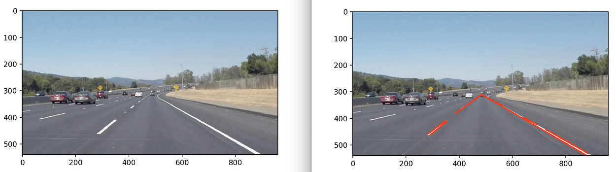
We've got our original image, but now we've sprinkled in those detected lines as a fancy overlay. 📸✨
But hold on, we're not done yet. We want to be able to tell apart the left and right lane lines and show just one line for each. 🛣️🚗
So, in the next part, we're going to work some magic and create a single line for each bunch of detected lane markings. 🪄
📕Creating a Single Left and Right Lane Line
The final step in our pipeline will be to create only one line for each of the groups of lines we found in the last step. This can be done by fitting a simple linear model to the various endpoints of the line segments in each group, and then rendering a single overlay line on that linear model.
📗Grouping the Lines into Left and Right Groups
First things first, we have to figure out which lines go where. 🧐
In algebra class, you probably learned about slopes. 📈 Basically, it's all about how steep a line is. 🏔️
Imagine lines in a picture - like a road. 🛣️ If a line slopes upwards from left to right, that's a positive slope, like climbing a hill. ⬆️ But if it slopes downwards from left to right, that's a negative slope, like going downhill. ⬇️
Now, here's the twist. Our picture is a bit different because it starts from the top left. 🧭 So, negative slopes go up, and positive slopes go down in our world. 🌍
For our job, the lines on the left side of the road have negative slopes, going up toward the horizon. 👈 And the lines on the right have positive slopes, going down towards the bottom of the picture. 👉
But wait, there's more! We only care about lines that are pretty steep - not too horizontal. We want them to be almost vertical or really slanted. 🕶️ So, any line with a slope less than 0.5 is a no-go.
That's the plan! We'll sort 'em out by looking at their slopes and make our road-detecting life easier. 🚗💨
import math


left_line_x = []
left_line_y = []
right_line_x = []
right_line_y = []
for line in lines:
    for x1, y1, x2, y2 in line:
        slope = (y2 - y1) / (x2 - x1) # <-- Calculating the slope.
        if math.fabs(slope) < 0.5: # <-- Only consider extreme slope
            continue
        if slope <= 0: # <-- If the slope is negative, left group.
            left_line_x.extend([x1, x2])
            left_line_y.extend([y1, y2])
        else: # <-- Otherwise, right group.
            right_line_x.extend([x1, x2])
            right_line_y.extend([y1, y2])
In this code, we loop over all of the lines we’ve detected and calculate their slope. If the slope is not extreme enough to be a lane marking edge, we will not consider it at all, and continue the loop without handling that line. If the slope is negative, the line belongs to the left lane markings group. If the slope is positive, the line belongs to the right group. To add a line to either group, we add the various x and y endpoint coordinates to lists for each side.
📗Creating a Single Linear Representation of each Line Group
🚗 Our second challenge in making a single line is to blend the lines in each group nicely in the picture. 😌
🤔 To do that, let's think about some things we already know. Like, the top and bottom points of both lane lines have the same height (y-values). We want these lines to start at the bottom of the picture, follow the road markings, and stop just below the horizon. 🌅
📐 So, the tricky part is figuring out the right side-to-side position (x-values) for each point on these two lines. 🧐
min_y = image.shape[0] * (3 / 5) # <-- Just below the horizon
max_y = image.shape[0] # <-- The bottom of the image
🤓 To find the right sideways spots (x-values) for the top and bottom points of our lines, we can use math, but don't worry, it's not too hard! 🤔
📐 We create two special functions 📈, one for the left line and one for the right. These functions help us figure out the x-values based on the y-values. 🧮
🔍 Then, we just plug in those common y-values we know, and bam! We get the x-values we need for our lines. 🎯
🤖 Luckily, numpy has some handy tools 🧰, like "polyfit" and "poly1d," that do this for us. They make linear functions that match our points perfectly. 🙌
Now we can use these lines as our input to the draw_lines function in our pipeline:
import cv2
import numpy as np
import matplotlib.pyplot as plt
import math

def region_of_interest(img, vertices):
    mask = np.zeros_like(img)
    cv2.fillPoly(mask, vertices, 255)
    masked_img = cv2.bitwise_and(img, mask)
    return masked_img

def draw_lines(img, lines, color=[255, 0, 0], thickness=3):
    if lines is None:
        return
    img_copy = np.copy(img)
    line_img = np.zeros(
        (
            img.shape[0],
            img.shape[1],
            3
        ),
        dtype=np.uint8,
    )
    for line in lines:
        x1, y1, x2, y2 = line[0]
        slope = (y2 - y1) / (x2 - x1)
        if math.fabs(slope) < 0.5:
            continue
        if slope <= 0:
            left_line_x.extend([x1, x2])
            left_line_y.extend([y1, y2])
        else:
            right_line_x.extend([x1, x2])
            right_line_y.extend([y1, y2])

    min_y = img.shape[0] * (3 / 5)
    max_y = img.shape[0]

    poly_left = np.poly1d(np.polyfit(
        left_line_y,
        left_line_x,
        deg=1
    ))
    left_x_start = int(poly_left(max_y))
    left_x_end = int(poly_left(min_y))
    poly_right = np.poly1d(np.polyfit(
        right_line_y,
        right_line_x,
        deg=1
    ))
    right_x_start = int(poly_right(max_y))
    right_x_end = int(poly_right(min_y))

    line_image = np.copy(img)  # Create a copy to draw lines on
    cv2.line(line_image, (left_x_start, int(max_y)), (left_x_end, int(min_y)), color, thickness)
    cv2.line(line_image, (right_x_start, int(max_y)), (right_x_end, int(min_y)), color, thickness)

    img_result = cv2.addWeighted(img_copy, 0.8, line_image, 1.0, 0.0)
    return img_result

# Load the image
image = cv2.imread('sample.jpg')
image = cv2.cvtColor(image, cv2.COLOR_BGR2RGB)

plt.figure(figsize=(8, 6))

# Define the region of interest vertices
region_of_interest_vertices = [(0, image.shape[0]), (image.shape[1] / 2, image.shape[0] / 2), (image.shape[1], image.shape[0])]

# Convert to grayscale
gray_image = cv2.cvtColor(image, cv2.COLOR_RGB2GRAY)

# Apply Canny edge detection
cannyed_image = cv2.Canny(gray_image, 100, 200)

# Apply region of interest mask
cropped_image = region_of_interest(cannyed_image, np.array([region_of_interest_vertices], np.int32))

# Perform Hough Line Transform
lines = cv2.HoughLinesP(
    cropped_image,
    rho=6,
    theta=np.pi / 60,
    threshold=160,
    lines=np.array([]),
    minLineLength=40,
    maxLineGap=25
)

left_line_x = []
left_line_y = []
right_line_x = []
right_line_y = []

# Extract and classify lines
for line in lines:
    x1, y1, x2, y2 = line[0]
    slope = (y2 - y1) / (x2 - x1)
    if math.fabs(slope) < 0.5:
        continue
    if slope <= 0:
        left_line_x.extend([x1, x2])
        left_line_y.extend([y1, y2])
    else:
        right_line_x.extend([x1, x2])
        right_line_y.extend([y1, y2])

# Draw and overlay the detected lane lines
line_image = draw_lines(
    image,
    [[
        [left_x_start, max_y, left_x_end, min_y],
        [right_x_start, max_y, right_x_end, min_y],
    ]],
    thickness=5,
)

# Display the result
plt.imshow(line_image)
plt.show()
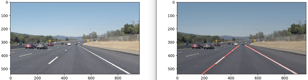
We did it!!!
📕Level Up: Land Detection for a Video
📹 Now, let's take all the cool stuff we've done so far and put it in a neat little function called "pipeline()"! 🚀
So, this function will do all the magic on a video and slap those lane lines right on it! 🛣️
Just give it a video, and it'll work its magic. 🎩
import matplotlib.pyplot as plt
import matplotlib.image as mpimg
import numpy as np
import cv2
import math
def region_of_interest(img, vertices):
    mask = np.zeros_like(img)
    match_mask_color = 255
    cv2.fillPoly(mask, vertices, match_mask_color)
    masked_image = cv2.bitwise_and(img, mask)
    return masked_image
def draw_lines(img, lines, color=[255, 0, 0], thickness=3):
    line_img = np.zeros(
        (
            img.shape[0],
            img.shape[1],
            3
        ),
        dtype=np.uint8
    )
    img = np.copy(img)
    if lines is None:
        return
    for line in lines:
        for x1, y1, x2, y2 in line:
            cv2.line(line_img, (x1, y1), (x2, y2), color, thickness)
    img = cv2.addWeighted(img, 0.8, line_img, 1.0, 0.0)
    return img
def pipeline(image):
    """
    An image processing pipeline which will output
    an image with the lane lines annotated.
    """
    height = image.shape[0]
    width = image.shape[1]
    region_of_interest_vertices = [
        (0, height),
        (width / 2, height / 2),
        (width, height),
    ]
    gray_image = cv2.cvtColor(image, cv2.COLOR_RGB2GRAY)
    cannyed_image = cv2.Canny(gray_image, 100, 200)

    cropped_image = region_of_interest(
        cannyed_image,
        np.array(
            [region_of_interest_vertices],
            np.int32
        ),
    )

    lines = cv2.HoughLinesP(
        cropped_image,
        rho=6,
        theta=np.pi / 60,
        threshold=160,
        lines=np.array([]),
        minLineLength=40,
        maxLineGap=25
    )

    left_line_x = []
    left_line_y = []
    right_line_x = []
    right_line_y = []

    for line in lines:
        for x1, y1, x2, y2 in line:
            slope = (y2 - y1) / (x2 - x1)
            if math.fabs(slope) < 0.5:
                continue
            if slope <= 0:
                left_line_x.extend([x1, x2])
                left_line_y.extend([y1, y2])
            else:
                right_line_x.extend([x1, x2])
                right_line_y.extend([y1, y2])
    min_y = int(image.shape[0] * (3 / 5))
    max_y = int(image.shape[0])
    poly_left = np.poly1d(np.polyfit(
        left_line_y,
        left_line_x,
        deg=1
    ))

    left_x_start = int(poly_left(max_y))
    left_x_end = int(poly_left(min_y))

    poly_right = np.poly1d(np.polyfit(
        right_line_y,
        right_line_x,
       deg=1
    ))

    right_x_start = int(poly_right(max_y))
    right_x_end = int(poly_right(min_y))
    line_image = draw_lines(
        image,
        [[
            [left_x_start, max_y, left_x_end, min_y],
            [right_x_start, max_y, right_x_end, min_y],
        ]],
        thickness=5,
    )
    return line_image
Then we can write a video processing pipeline:
import cv2
import numpy as np

# Define the video input and output filenames
input_video = 'HighWayRoadSample.mp4'
output_video = 'HighWayRoadSample_output.mp4'

# Initialize video capture
cap = cv2.VideoCapture(input_video)

# Get the video's frame dimensions and create a VideoWriter object for the output video
fps = int(cap.get(cv2.CAP_PROP_FPS))
frame_width = int(cap.get(cv2.CAP_PROP_FRAME_WIDTH))
frame_height = int(cap.get(cv2.CAP_PROP_FRAME_HEIGHT))
out = cv2.VideoWriter(output_video, cv2.VideoWriter_fourcc(*'mp4v'), fps, (frame_width, frame_height))

# Load the lane detection pipeline code
# (Assuming you've already defined the pipeline function)

# Process each frame of the video
while True:
    ret, frame = cap.read()
    if not ret:
        break  # Break the loop at the end of the video

    # Apply the lane detection pipeline to the current frame
    processed_frame = pipeline(frame)

    # Write the processed frame to the output video
    out.write(processed_frame)

# Release video capture and writer objects
cap.release()
out.release()

# Close all OpenCV windows
cv2.destroyAllWindows()

print("Video processing complete.")
After the video is finished processing, you should be able to open your video and have it match very nearly to the one below. Congratulations!
Output:
Thank You so much for your valuable time.😊🥳👋
If you have any questions or comments, feel free to reach out to me :)
👋 Hi there! Let's connect and collaborate!
Here are some ways to reach me:
🔹 GitHub: github.com/mithindev
🔹 Twitter: twitter.com/MithinDev
🔹 LinkedIn: linkedin.com/in/mithindev
Looking forward to connecting with you!
PS: Ignore the hashes😊
#LaneDetection #ComputerVision #OpenCV #PythonProgramming #ImageProcessing #Algorithm #TechJourney #CodingTutorial #ComputerGraphics #EdgeDetection #HoughTransform #LaneMarkings #LaneDetectionAlgorithm #PythonCoding #ComputerScience #ProgrammingTips #VideoProcessing #ImageManipulation #Tutorial #CodeExamples #LaneDetectionTutorial #CVTools #MachineLearning #ArtificialIntelligence #DeepLearning #LaneDetectionCode #LaneDetectionProject #LaneDetectionPipeline #CodeTutorial #LaneMarkers #LaneDetectionGuide #TechExploration #ProgrammingJourney #CodingJourney